Quantum Information Processing
Quantum Circuit
The most common model for quantum computing is the quantum circuit model.
In QuTiP, we use QubitCircuit to represent a quantum circuit.
The circuit is characterized by registers and gates:
Registers: The argument
Nspecifies the number of qubit registers in the circuit and the argumentnum_cbits(optional) specifies the number of classical bits available for measurement and control.Gates: Each quantum gate is saved as a class object
Gatewith information such as gate name, target qubits and arguments. Gates can also be controlled on a classical bit by specifying the register number with the argumentclassical_controls.Measurements: We can also carry out measurements on individual qubit (both in the middle and at the end of the circuit). Each measurement is saved as a class object
Measurementwith parameters such as targets, the target qubit on which the measurement will be carried out, and classical_store, the index of the classical register which stores the result of the measurement.
A circuit with the various gates and registers available is demonstrated below:
from qutip_qip.circuit import QubitCircuit
from qutip_qip.operations.gates import X, CX, SWAP
from qutip_qip.operations.measurement import Mz
from qutip import tensor, basis

qc = QubitCircuit(2, num_cbits=1)

qc.add_gate(SWAP, targets=[0, 1])
qc.add_measurement(Mz, targets=[1], classical_store=0) # measurement gate
qc.add_gate(CX, controls=0, targets=1)
qc.add_gate(X, targets=0, classical_controls=[0]) # classically controlled gate
qc.add_gate(SWAP, targets=[0, 1])

print(qc.instructions)
Output:
  [GateInstruction(operation=Gate(SWAP, num_qubits=2), qubits=(0, 1), cbits=(), style=None, cbits_ctrl_value=None),
    MeasurementInstruction(operation= Measurement(M), qubits=(1,), cbits=(0,), style={}),
    GateInstruction(operation=Gate(CX, num_qubits=2), qubits=(0, 1), cbits=(), style=None, cbits_ctrl_value=None),
    GateInstruction(operation=Gate(X, num_qubits=1), qubits=(0,), cbits=(0,), style=None, cbits_ctrl_value=1),
    GateInstruction(operation=Gate(SWAP, num_qubits=2), qubits=(0, 1), cbits=(), style=None, cbits_ctrl_value=None)]
Unitaries
There are a few useful functions associated with the circuit object. For example,
the QubitCircuit.propagators() method returns a list of the unitaries associated
with the sequence of gates in the circuit. By default, the unitaries are expanded to the
full dimension of the circuit:
U_list = qc.propagators(ignore_measurement=True)
print(U_list[:-1])
Output:
[Quantum object: dims=[[2, 2], [2, 2]], shape=(4, 4), type='oper', dtype=Dense, isherm=True
Qobj data =
[[1. 0. 0. 0.]
 [0. 0. 1. 0.]
 [0. 1. 0. 0.]
 [0. 0. 0. 1.]], Quantum object: dims=[[2, 2], [2, 2]], shape=(4, 4), type='oper', dtype=Dense, isherm=True
Qobj data =
[[1. 0. 0. 0.]
 [0. 1. 0. 0.]
 [0. 0. 0. 1.]
 [0. 0. 1. 0.]], Quantum object: dims=[[2, 2], [2, 2]], shape=(4, 4), type='oper', dtype=CSR, isherm=True
Qobj data =
[[0. 0. 1. 0.]
 [0. 0. 0. 1.]
 [1. 0. 0. 0.]
 [0. 1. 0. 0.]], Quantum object: dims=[[2, 2], [2, 2]], shape=(4, 4), type='oper', dtype=Dense, isherm=True
Qobj data =
[[1. 0. 0. 0.]
 [0. 0. 1. 0.]
 [0. 1. 0. 0.]
 [0. 0. 0. 1.]]]
Another option is to only return the unitaries in their original dimension. This
can be achieved with the argument expand=False specified to the
QubitCircuit.propagators().
U_list = qc.propagators(expand=False, ignore_measurement=True)
print(U_list[:-1])
Output:
[Quantum object: dims=[[2, 2], [2, 2]], shape=(4, 4), type='oper', dtype=Dense, isherm=True
Qobj data =
[[1. 0. 0. 0.]
 [0. 0. 1. 0.]
 [0. 1. 0. 0.]
 [0. 0. 0. 1.]], Quantum object: dims=[[2, 2], [2, 2]], shape=(4, 4), type='oper', dtype=Dense, isherm=True
Qobj data =
[[1. 0. 0. 0.]
 [0. 1. 0. 0.]
 [0. 0. 0. 1.]
 [0. 0. 1. 0.]], Quantum object: dims=[[2], [2]], shape=(2, 2), type='oper', dtype=Dense, isherm=True
Qobj data =
[[0. 1.]
 [1. 0.]], Quantum object: dims=[[2, 2], [2, 2]], shape=(4, 4), type='oper', dtype=Dense, isherm=True
Qobj data =
[[1. 0. 0. 0.]
 [0. 0. 1. 0.]
 [0. 1. 0. 0.]
 [0. 0. 0. 1.]]]
Gates
The pre-defined gates for the class Gate are shown in the table below:
Gate name |
Description |
|---|---|
“X” |
Pauli-X gate |
“Y” |
Pauli-Y gate |
“Z” |
Pauli-Z gate |
“H” |
Hadamard gate |
“S” |
Single-qubit rotation or Z90 |
“Sdag” |
Inverse of S gate |
“T” |
Square root of S gate |
“Tdag” |
Inverse of T gate |
“SQRTX” |
Square root of X gate |
“SQRTXdag” |
Inverse of SQRTX gate |
“RX” |
Rotation around x axis |
“RY” |
Rotation around y axis |
“RZ” |
Rotation around z axis |
“PHASE” |
Adds a relative phase to ket 1 |
“R” |
Arbitrary single qubit rotation |
“QASMU” |
U rotation gate used as a primitive in the QASM standard |
“CX” |
(CNOT) Controlled X gate |
“CY” |
Controlled Y gate |
“CZ” |
Controlled Z gate |
“CH” |
Controlled H gate |
“CS” |
Controlled S gate |
“CSdag” |
Controlled Sdag gate |
“CT” |
Controlled T gate |
“CTdag” |
Controlled Tdag gate |
“CRX” |
Controlled rotation around x axis |
“CRY” |
Controlled rotation around y axis |
“CRZ” |
Controlled rotation around z axis |
“CPHASE” |
Controlled Phase gate |
“CQASMU” |
Controlled QASMU gate |
“SWAP” |
Swap the states of two qubits |
“ISWAP” |
Swap gate with additional phase for 01 and 10 states |
“ISWAPdag” |
Inverse of ISWAP gate |
“SQRTSWAP” |
Square root of the SWAP gate |
“SQRTSWAPdag” |
Inverse of SQRTSWAP gate |
“SQRTISWAP” |
Square root of the ISWAP gate |
“SQRTISWAPdag” |
Inverse of SQRTISWAP gate |
“BERKELEY” |
Berkeley gate |
“BERKELEYdag” |
Inverse of BERKELEY gate |
“SWAPALPHA” |
SWAPALPHA gate |
“MS” |
Mølmer-Sørensen gate |
“RZX” |
RZX gate |
“TOFFOLI” |
|
“FREDKIN” |
Fredkin gate |
“GLOBALPHASE” |
Global phase gate |
“IDENTITY” |
Identity gate |
For some of the gates listed above, QubitCircuit also has a primitive QubitCircuit.resolve_gates() method that decomposes them into elementary gate sets such as CX or SWAP with single-qubit gates (RX, RY and RZ). However, this method is not fully optimized. It is very likely that the depth of the circuit can be further reduced by merging quantum gates. It is required that the gate resolution be carried out before the measurements to the circuit are added.
Custom Gates
In addition to these pre-defined gates, QuTiP also allows the user to define their own gate.
The following example shows how to define a customized gate.
The key step is to define a
gate function returning a qutip.Qobj and save it in the attribute user_gates.
Note
Available from QuTiP 4.4
from qutip_qip.operations import Gate, rx

def user_gate1(arg_value):
     # controlled rotation X
     mat = np.zeros((4, 4), dtype=np.complex128)
     mat[0, 0] = mat[1, 1] = 1.
     mat[2:4, 2:4] = rx(arg_value).full()
     return Qobj(mat, dims=[[2, 2], [2, 2]])


def user_gate2():
     # S gate
     mat = np.array([[1.,   0],
                     [0., 1.j]])
     return Qobj(mat, dims=[[2], [2]])

qc = QubitCircuit(2)
# qubit 0 controls qubit 1
qc.add_gate("CRX", controls=[0], targets=[1], arg_value=np.pi/2)

# qubit 1 controls qubit 0
qc.add_gate("CRX", controls=[1], targets=[0], arg_value=np.pi/2)

# we also add a gate using a predefined Gate object
qc.add_gate("S", targets=[1])
props = qc.propagators()

print(props[0])
Output:
Quantum object: dims=[[2, 2], [2, 2]], shape=(4, 4), type='oper', dtype=Dense, isherm=False
Qobj data =
  [[1.     +0.j      0.     +0.j      0.     +0.j      0.     +0.j     ]
   [0.     +0.j      1.     +0.j      0.     +0.j      0.     +0.j     ]
   [0.     +0.j      0.     +0.j      0.70711+0.j      0.     -0.70711j]
   [0.     +0.j      0.     +0.j      0.     -0.70711j 0.70711+0.j     ]]
print(props[1])
Output:
Quantum object: dims=[[2, 2], [2, 2]], shape=(4, 4), type='oper', dtype=Dense, isherm=False
Qobj data =
[[1.     +0.j      0.     +0.j      0.     +0.j      0.     +0.j     ]
 [0.     +0.j      0.70711+0.j      0.     +0.j      0.     -0.70711j]
 [0.     +0.j      0.     +0.j      1.     +0.j      0.     +0.j     ]
 [0.     +0.j      0.     -0.70711j 0.     +0.j      0.70711+0.j     ]]
print(props[2])
Output:
  Quantum object: dims=[[2, 2], [2, 2]], shape=(4, 4), type='oper', dtype=CSR, isherm=False
  Qobj data =
  [[1.+0.j 0.+0.j 0.+0.j 0.+0.j]
   [0.+0.j 0.+1.j 0.+0.j 0.+0.j]
   [0.+0.j 0.+0.j 1.+0.j 0.+0.j]
   [0.+0.j 0.+0.j 0.+0.j 0.+1.j]]
Plotting Quantum Circuits
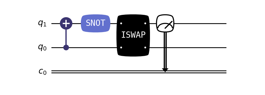
QuTiP-QIP offers three distinct methods for visualizing quantum circuits. Below is an example that demonstrates how to create and plot a quantum circuit using these methods:
Matplotlib (Default):
from qutip_qip.circuit import QubitCircuit
from qutip_qip.operations.gates import H, CX, ISWAP
from qutip_qip.operations.measurement import Mz

# create the quantum circuit
qc = QubitCircuit(2, num_cbits=1)
qc.add_gate(CX, controls=0, targets=1)
qc.add_gate(H, targets=1)
qc.add_gate(ISWAP, targets=[0,1])
qc.add_measurement(Mz, targets=1, classical_store=0)

qc.draw("matplotlib", dpi=300)
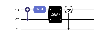
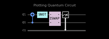
Customization Examples:
from qutip_qip.circuit import QubitCircuit
from qutip_qip.operations.gates import H, CX, ISWAP
from qutip_qip.operations.measurement import Mz

# create the quantum circuit
qc = QubitCircuit(2, num_cbits=1)
qc.add_gate(CX, controls=0, targets=1)
qc.add_gate(H, targets=1)
qc.add_gate(ISWAP, targets=[0,1])
qc.add_measurement(Mz, targets=1, classical_store=0)

qc.draw("matplotlib", bulge=False, theme='dark', title="Plotting Quantum Circuit", dpi=300)

Customization Parameters
Parameter
Description
dpi : int = 150DPI of the figure.
fontsize : int = 10Fontsize control at the circuit level, including tile and wire labels.
end_wire_ext : int = 2Extension of the wire at the end of the circuit.
padding : float = 0.3Padding between the circuit and the figure border.
gate_margin : float = 0.15Margin space left on each side of the gate.
wire_sep : float = 0.5Separation between the wires.
layer_sep : float = 0.5Separation between the layers.
gate_pad : float = 0.05Padding between the gate and the gate label.
label_pad : float = 0.1Padding between the wire label and the wire.
bulge : Union[str, bool] = TrueBulge style of the gate. Renders non-bulge gates if False.
align_layer : bool = FalseAlign the layers of the gates across different wires.
theme : Optional[Union[str, Dict]] = "qutip"Color theme of the circuit. Available themes are ‘qutip’, ‘light’, ‘dark’ and ‘modern’.
title : Optional[str] = NoneTitle of the circuit.
bgcolor : Optional[str] = NoneBackground color of the circuit.
color : Optional[str] = NoneControls color of accent elements (e.g., cross sign in the target node) and sets as default color of gate-label. Can be overwritten by gate-specific color.
wire_label : Optional[List] = NoneLabels of the wires.
wire_color : Optional[str] = NoneColor of the wires.
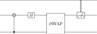
Text:
from qutip_qip.circuit import QubitCircuit
from qutip_qip.operations.gates import H, CX, ISWAP
from qutip_qip.operations.measurement import Mz

# create the quantum circuit
qc = QubitCircuit(2, num_cbits=1)
qc.add_gate(CX, controls=0, targets=1)
qc.add_gate(H, targets=1)
qc.add_gate(ISWAP, targets=[0,1])
qc.add_measurement(Mz, targets=1, classical_store=0)

qc.draw("text")
         ┌────┐  ┌───┐  ┌───────┐  ┌───┐
  q1 :───┤ CX ├──┤ H ├──┤       ├──┤ M ├───
         └──┬─┘  └───┘  │       │  └─╥─┘
            │           │       │    ║
  q0 :──────█───────────┤ ISWAP ├────║─────
                        └───────┘    ║
                                     ║
  c0 :═══════════════════════════════╩═════
Customization Parameters
Parameter
Description
gate_pad : int = 1Padding between the gate and the gate label.
wire_label : Optional[List] = NoneLabels of the wires.
align_layer : bool = FalseAlign the layers of the gates across different wires.
end_wire_ext : int = 2Extension of the wire at the end of the circuit.
LaTeX:
A quantum circuit (described above) can directly be plotted using the QCircuit library (https://github.com/CQuIC/qcircuit). QCircuit is a quantum circuit drawing application and is implemented directly into QuTiP.
More information related to installing these packages is also available in the installation guide (Additional software for Plotting Circuits).
An example code for plotting the example quantum circuit from above is given:
from qutip_qip.circuit import QubitCircuit
from qutip_qip.operations.gates import H, CX, ISWAP
from qutip_qip.operations.measurement import Mz

# create the quantum circuit
qc = QubitCircuit(2, num_cbits=1)
qc.add_gate(CX, controls=0, targets=1)
qc.add_gate(H, targets=1)
qc.add_gate(ISWAP, targets=[0,1])
qc.add_measurement(Mz, targets=1, classical_store=0)

qc.draw("latex")
Circuit simulation
There are two different ways to simulate the action of quantum circuits using QuTiP:
The first method utilizes unitary application through matrix products on the input states. This method simulates circuits exactly in a deterministic manner. This is achieved through
CircuitSimulator. A short guide to exact simulation can be found at Gate-level circuit simulation. The teleportation notebook is also useful as an example.A different method of circuit simulation employs driving Hamiltonians with the ability to simulate circuits in the presence of noise. This can be achieved through the various classes in
device.A short guide to processors for QIP simulation can be found at Pulse-level circuit simulation.